Published by K12 Handhelds, Inc.
www.k12handhelds.com
Phone: 800-679-2226
Copyright © 2006 by K12 Handhelds, Inc. License CC-by, 
This work is licensed under a Creative Commons Attribution 3.0 United States License.
Table of Contents
Gathering and Graphing Data
Statistics is a kind of math that involves the collection and analysis of data. Many jobs use statistics – teachers, insurance agents, sports coaches, and sociologists all use statistics every day.
The first step of using statistics is to gather the data. A teacher might need to gather data about the scores students got on a recent test. A coach might need to get data on how the players on an opposing team are performing.
On common way to gather and record data is with a tally sheet and a frequency table. A frequency table looks like this:
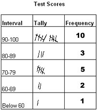
The column marked interval tells the grouping or range of data. In this case, the data is being recorded according to the range of scores. Students who got a score of 90 or higher are recorded in the first row. Students with a score between 80 and 89 are recorded in the second row, etc.
In the column marked tally, the person recording the data makes a mark in the appropriate box for each piece of data they record.
When this is finished, the number of tally marks in each interval are added and the total is written in the column marked frequency. The frequency is the number of occurrences for each interval or the number of times something happened. For example, the frequency of 10 in the first row tells that 10 students got a score of 90-100.
After the frequencies are figured out, people often want a nice way to show the data. Graphing is one way to do this. There are many types of graphs. The type of graph that is used depends on the data and which graph will show the information best.
One type of graph is a bar graph. This is a bar graph of the test score data from our frequency table:
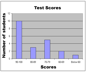
When creating or reading a bar graph, the graph is read just like a coordinate plane. (See the ebook on Coordinate Planes for a review of this.) Use the x-axis and y-axis to interpret the data.
Data can also be represented in a circle graph. This is also called a pie chart. Here is a pie chart for the test score data:
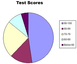
In a pie chart, the full circle is the total (100% of the data). The frequency count for each interval is then figured out as a percentage of the total. For example, in our test score data, the total number of students is 21. (This is the sum of all the frequencies: 10 + 3 + 5 + 2 + 1.)
To figure out the percentage of students that scored between 90 and 100, we divide the total by that frequency:
10 ÷ 21 = .48 or 48%
In the pie chart then, 48% of the full circle is colored for the interval 90-100.
This same process is followed for each interval to make the pie chart.
Measures of Central Tendency
When looking at statistics, people often want to know what the data shows. For example, what was the average score the students got? What was the highest score? What was the lowest score? When looking at sports statistics, a coach might want to know how many points the other team usually scores. Who is their highest scorer?
To answer these questions, we need to look at measures of central tendency. These are numbers that tell us things like the average, the range of data, and the middle number. There are several different measures of central tendency. Let’s look at each one.
Mean
The mean is a simple average of a series.
To calculate the mean or average, add all the numbers together and divide by the number of items in the list.
For example, let’s figure out the mean of the total points scored by a team over their last five games. Here is the data:
Game 1 67 points scored
Game 2 52 points scored
Game 3 66 points scored
Game 4 40 points scored
Game 5 58 points scored
To calculate the mean, we first need to add all the numbers together.
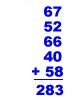
Then we divide by the number of items, in this case 5.
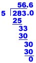
The mean or average is 56.6.
Now, you try calculating the average for these examples:
1. Find the average of: 8, 7, 10, 12, 11, 9, 6
2. Find the mean of: 98, 80, 94, 82
Median
Another measure of central tendency is the median. The median is the middle number in a series.
To calculate the median, arrange the numbers in order from lowest to highest and find the one in the middle. (If there is an even number of figures, take an average of the middle two.)
Let’s figure the median for the scores we looked at above:
Game 1 67 points scored
Game 2 52 points scored
Game 3 66 points scored
Game 4 40 points scored
Game 5 58 points scored
First, we need to arrange the numbers in order from lowest to highest.
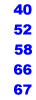
Then we need to find the one in the middle.
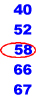
For this set of data, 58 is the median score.
3. Find the median for this set of data: 48, 32, 87, 64, 112, 60, 67
Mode
Another measure of central tendency is the mode. The mode is the most repeated number in a series.
To calculate the mode, list all the numbers in order and find the one that appears the most times.
Let’s find the mode for this data set: 80, 75, 90, 84, 90, 75, 60, 80, 91, 75
First, we need to arrange the numbers in order.
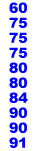
Then we need to find the one that shows up the most times.
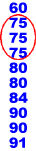
For this set of data, 75 is the mode.
4. Now, you find the mode for this set of data: 5, 4, 12, 6, 4, 4, 3, 2, 8, 6, 4, 5, 6, 5
Range
The final measure of central tendency we’ll look at is the range. The range is the difference between the highest and lowest number in a series.
To calculate the range, we again need to arrange the numbers in order from lowest to highest and then subtract the lowest from the highest.
Let’s find the range for the data set we looked at before:
80, 75, 90, 84, 90, 75, 60, 80, 91, 75
First, we need to arrange the numbers in order.
Then we need to subtract the lowest number from the highest number.

For this set of data, the range is 31
Now, you try one.
5. Find the range for this data: 76, 85, 92, 77, 88, 85
Probability
One use of statistics is to predict the chances that something might happen. Probability is the likelihood that something might happen. If something is guaranteed to happen, the probability is 1. If it is impossible to happen, the probability is 0. If it is not guaranteed or impossible, the probability is somewhere between 0 and 1.
To figure out probability, we need to look at outcomes. Outcomes are all the possible things that might happen. For example, if we flip a coin, one outcome is heads. Another outcome is tails. Those are the only two possibilities, so there are two possible outcomes.
If we want to know the probability of one particular outcome, that is called a favorable outcome. If we want to know how many times flipping a coin will result in heads, the favorable outcome is heads. There is one favorable outcome.
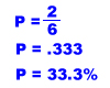
Here is the formula to calculate probability:
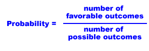
Let’s apply this to flipping a coin. What is the probability of getting heads? We know that there is one favorable outcome (heads) and two possible outcomes (heads and tails), so:
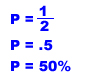
Generally, we convert probabilities to percentages as we did here. (See the ebook on Decimals for a review on percentages.)
Let’s do another example. There is a spinner with spots for the numbers 1 through 6. When you spin, what is the probability you will get a 2 or a 4?
First, we need to figure out the number of possible outcomes and probable outcomes. Since there are 6 different numbers you might get, the number possible outcomes is 6. We want to know the change of getting a 2 or a 4. Those are the probable outcomes, and there are to. So here is how we figure out the probability:
Here’s one for you to try.
6. There is a bag of marbles. It has 3 blue marbles and 9 black marbles. If you draw one without looking, what is the chance you will get a blue marble?
Combinations
When there are a large number of possible combinations of outcomes, it is helpful to have a way to figure out how many there are. One way is to draw a picture. We can use a tree diagram to do this.
Suppose you are choosing an outfit. You have four pairs of jeans and three sweaters. How many different outfits can you make?
Let’s draw a tree diagram with branches to show each possibility:
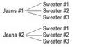
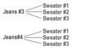
If we count all the resulting options, there are 12 different outfits that can be made.
A short cut to figuring out the number of total combinations is the Counting Principle. The Counting Principle says that to find the number of different outcomes of multiple items, you multiply the number of outcomes for each item times the number of items.
For example, in our example of four jeans and three sweaters, the number of possible outcomes is:
(3)(4) = 12
This is the same answer we came up with using the tree diagram.
Let’s do another one.
Suppose you are buying a new skateboard. There are 6 different kinds of wheels you can choose from. The skateboard you want comes in 10 different colors. How many different combinations of choices do you have?
Using the Counting Principle, we multiply the number of choices for one item times the number of choices for the other.
(6)(10) = 60
You have 60 different combinations to choose from!
Now, you try a couple.
7. You’re ordering a pizza special with one topping. There are five different choices of toppings. You can get the pizza with thick or thin crust. How many different combinations of pizza are there?
8. Brian is making an ice cream sundae for his mother. They have chocolate, vanilla, and strawberry ice cream. They also have hot fudge, marshmallow, pineapple, and butterscotch topping. If his mother wants one flavor of ice cream and one kind of topping, how many combinations does she have to choose from?
Permutations
In the above examples of combinations, the order of the items or events didn’t matter. There are some arrangements though, where the order is important. When the order is important, the number of possibilities is called a permutation.
Let’s look at an example. There are four students, Julio, Angela, Adam, and Shanna. They are lining up to go to lunch. How many different orders are possible?
This is a permutation because order is important.
Let’s list out all the possible orders:
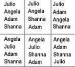
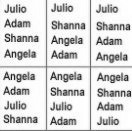
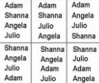
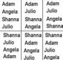
If you count out all the different permutations, there are 24.
That’s a lot of work to list those all out! Fortunately, there is a short cut. We can figure out the number of permutations using something called factorials.
Factorials are written with an exclamation point, such as:
4!
This is said “four factorial”.
A factorial of a number is the number times all positive integers smaller than the number. For example:
4! = 4 • 3 • 2 • 1
= 24
This is the number of permutations for 4 different items, as we found above.
So, the number of permutations of x things is x! (That’s x factorial.)
Let’s do another example.
Becky needs to make a secret password out of these letters and numbers:
A B C 1 2 3
She must use each character and can only use each one once. How many different choices does she have?
The order is important here, so we need figure out the number of permutations. There are 6 different characters, so our answer is:
= 6!
= 6 • 5 • 4 • 3 • 2 • 1
= 720
She has 720 different choices.
Now, you try a few.
9. There are 5 cars that need to get on the ferry. How many different orders are possible for the line of cars?
10. The four high school bands that are going to be in a parade. How many different arrangements are possible?